arXiv 2026
Learning Anisotropic Prediction Targets for Flow Models
State-of-the-art Pixel DiTs free of patch artifacts, without conv layers, even in 8-bit.
arXiv 2026
State-of-the-art Pixel DiTs free of patch artifacts, without conv layers, even in 8-bit.
Flow-based generative models are trained on a hand-chosen prediction target, such as the velocity, the noise, or the clean data. This choice strongly affects training and sample quality. We introduce Anisotropic Flow Models (AnisoFlow), which replaces a fixed prediction target with a fully learnable one. AnisoFlow learns to scale the noise component of the target anisotropically, assigning a separate nonnegative weight to each direction in a jointly learned basis. A closed-form map recovers the velocity from the network's prediction, leaving the architecture, flow-matching loss, and sampler unchanged. Since recovery is exact, training optimizes the target purely to make it easier for the network to predict. We theoretically analyze the resulting prediction error and predict that the preferred noise weight in each direction scales near-linearly with data variance, in agreement with the weights learned empirically in pixel space. AnisoFlow improves FID from 1.90 to 1.55 over the JiT baseline on ImageNet 256×256, by learning only the prediction target, without representation alignment or architectural changes. In pixel-space text-to-image generation, AnisoFlow improves image quality and, through better-conditioned velocity recovery, largely removes patch-seam artifacts under reduced-precision inference.
Same JiT-H/16 network and training recipe. Learning only the prediction target substantially improves FID, with no REPA, extra pretraining, or architectural changes.
A well-conditioned learned target fixes the patch seams of \(x\)-prediction pixel DiTs without extra conv layers, and stays clean even under INT8 and FP8 inference.
Flow models can predict targets like clean data \(x\), noise \(\epsilon\), or velocity \(u = \epsilon - x\). This is one of the most critical design choices, yet it remains largely empirical, often hand-picked or tuned within restricted degrees of freedom.
AnisoFlow makes this choice fully learnable. It defines a generic linear target \(u_W = W\epsilon - x\), where \(W\) is a learned positive semidefinite operator. A single \(W\), shared across tokens, scales the noise component in the target anisotropically.
A closed-form formula recovers the per-token velocity \(\hat{u}\) from the prediction \(\hat{u}_W\), so the network and \(W\) are jointly trained with the standard flow-matching loss on the recovered velocity, and sampling is unchanged.
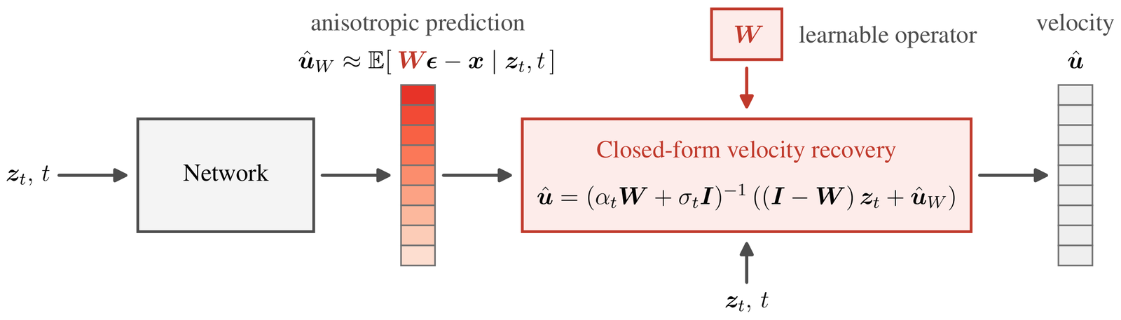
The network predicts the AnisoFlow target \(u_W = W\epsilon - x\), and a closed-form map recovers the standard velocity.
Writing \(W = B\,\mathrm{diag}(w_1, \dots, w_D)\,B^\top\) with an orthonormal basis \(B\), each direction \(i\) gets its own noise weight \(w_i \ge 0\). Clean-data prediction (\(w_i = 0\)), velocity prediction (\(w_i = 1\)), scalar interpolations (\(w_i \equiv w\)), and the binary low-rank mask of AsymFlow (\(w_i \in \{0, 1\}\)) are all special cases with restricted weight profiles. AnisoFlow instead learns the full profile together with the basis.
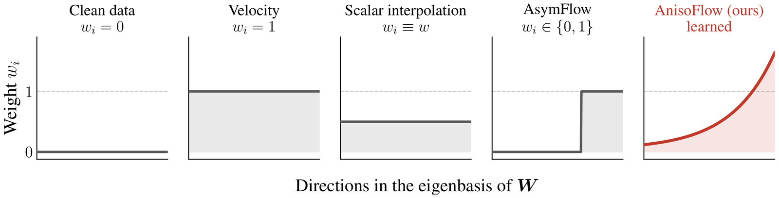
Standard targets correspond to restricted noise-weight profiles. AnisoFlow learns an unrestricted nonnegative profile across directions.
A larger noise weight reduces how much prediction error is amplified when converting back to velocity, but puts more noise into the target that the network has to predict. Analyzing this trade-off in the PCA basis, we predict that the preferred weight in each direction scales near-linearly with the data variance \(\lambda_i\), i.e., \(w_i \approx c\lambda_i\), and that a single weight profile suffices across all timesteps.
The trained pixel-space models agree with our theory. Regardless of initialization and basis optimization, the learned weights follow the near-linear scaling, and a basis learned from scratch aligns closely with PCA.
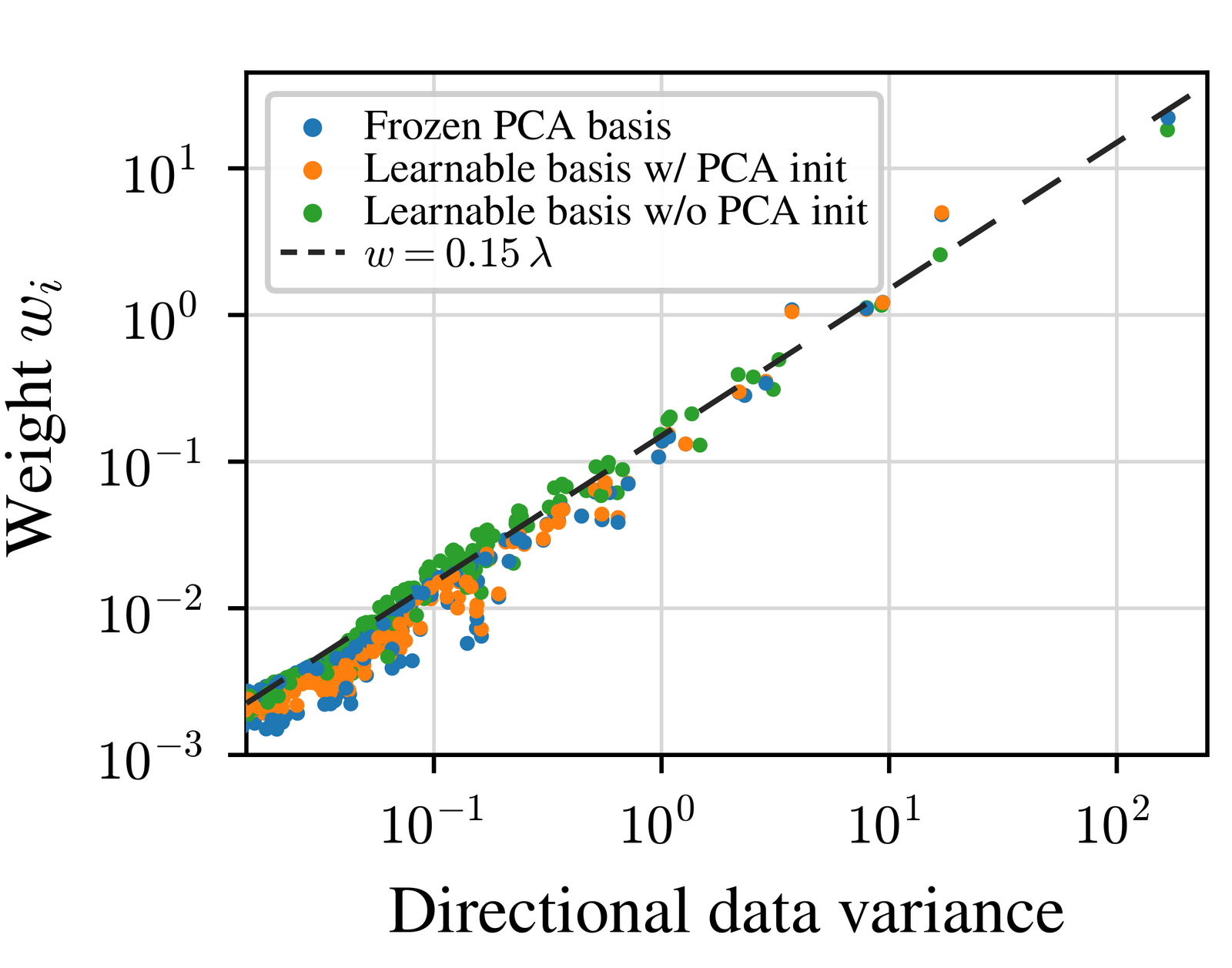
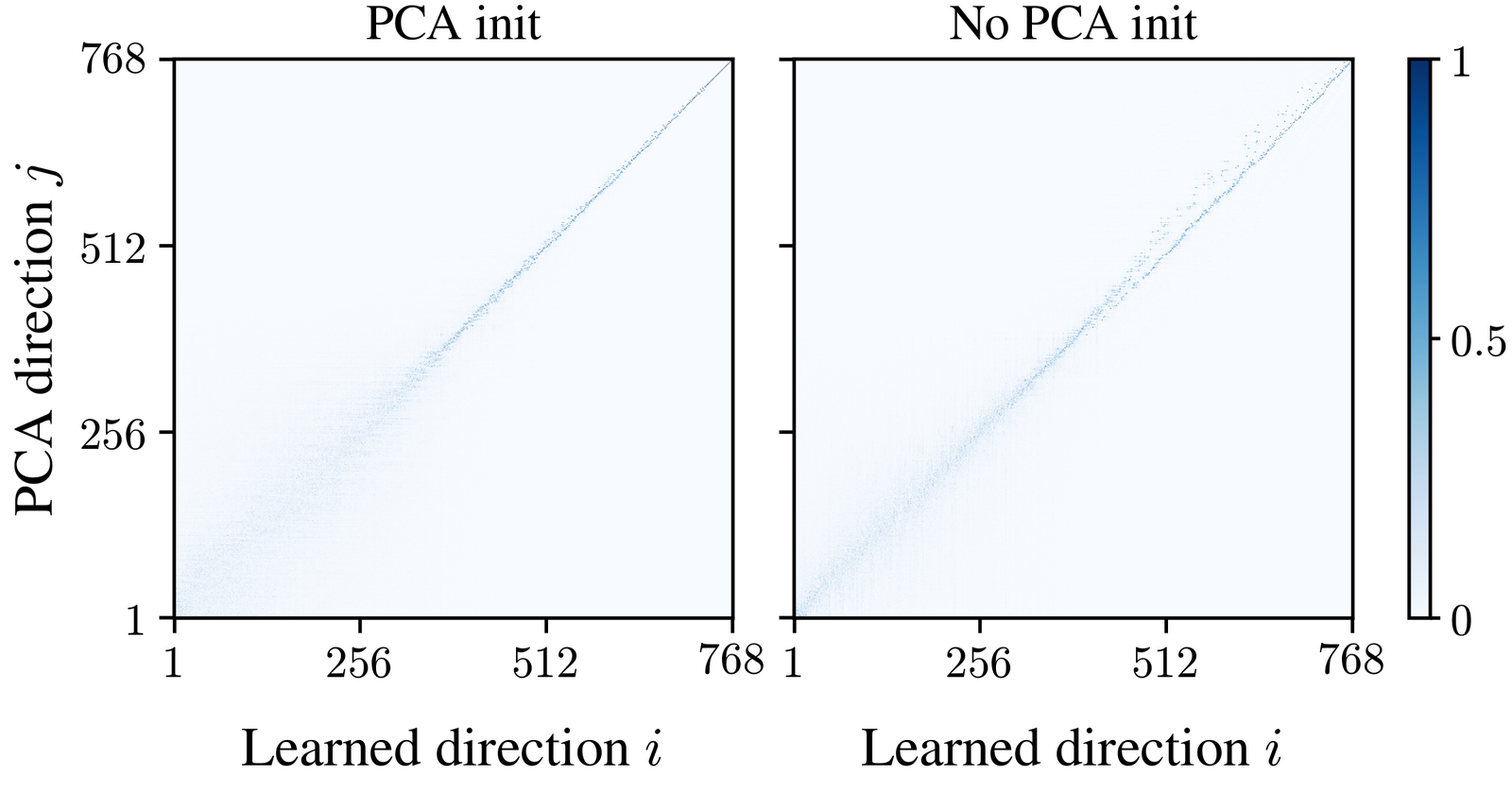
(a) Learned weights versus directional data variance on JiT-H/16. (b) Absolute inner products between PCA directions and learned directions. Both initializations yield near-diagonal alignment.
The baseline is JiT-H/16, a plain pixel transformer with \(x\)-prediction. AnisoFlow keeps the same network and training recipe and changes only the prediction target, with no REPA, pretrained encoder, or extra pretraining.
| Method | Noise weights | Noise basis | Init | FID↓ 160 epochs |
FID↓ 600 epochs |
|---|---|---|---|---|---|
| JiT | Frozen (zeros) | - | - | 2.68 | 1.90 |
| AsymFlow | Frozen (binary) | Frozen (PCA) | PCA | 2.34 | 1.76 |
| AnisoFlow | |||||
| AnisoFlow | Learned | Frozen (PCA) | PCA | 2.25 | 1.63 |
| AnisoFlow | Learned | Learned | PCA | 2.28 | 1.63 |
| AnisoFlow | Learned | Learned | - | 2.30 | 1.55 |
Learning continuous weights in a frozen PCA basis already improves considerably over JiT and AsymFlow. Learning the basis from an isotropic initialization gives the best final FID.
| Method | Target | Params | GFLOPs | FID↓ |
|---|---|---|---|---|
| Hierarchical CNNs (U-Net-like) | ||||
| ADM-G | \(\epsilon\) | 554M | 2240 | 4.59 |
| Hierarchical transformers (U-ViT-like) | ||||
| RIN | \(\epsilon\) | 320M | 668 | 3.42 |
| SiD, UViT/2 | \(\epsilon\) | 2B | 1110 | 2.44 |
| VDM++, UViT/2 | \(\epsilon\) | 2B | 1110 | 2.12 |
| SiD2, UViT/2 | \(\epsilon\) | - | 274 | 1.73 |
| PixelU-H/16† | \(x\) | 1.2B | 274 | 1.63* |
| EPG-G/16† | \(x\) | 1.4B | 642 | 1.58 |
| SiD2, UViT/1 | \(\epsilon\) | - | 1306 | 1.38 |
| Hierarchical transformers (DDT-like) | ||||
| PixNerd-XL/16† | \(\epsilon - x\) | 700M | 268 | 2.15 |
| DiP-XL/16† | \(\epsilon - x\) | 631M | - | 1.79 |
| DeCo-XL/16† | \(\epsilon - x\) | 682M | 245 | 1.62 |
| PixelDiT-XL/16† | \(\epsilon - x\) | 797M | 311 | 1.61 |
| FrequencyBooster-H/16† | \(x\) | 1.1B | - | 1.60* |
| HyperDiT-H† | \(\epsilon - x\) | 952M | 458 | 1.56* |
| Method | Target | Params | GFLOPs | FID↓ |
|---|---|---|---|---|
| Plain transformers (DiT-like) | ||||
| PixelFlow-XL/4 | \(\epsilon - x\) | 677M | 5818 | 1.98 |
| JiT-H/16 | \(x\) | 953M | 364 | 1.86* |
| PixelGen-XL/16† | \(x\) | 676M | 260 | 1.83 |
| JiT-G/16 | \(x\) | 2B | 766 | 1.82* |
| PixelREPA-H/16† | \(x\) | 953M | 364 | 1.81* |
| AsymFlow-H/16† | \(P\epsilon - x\) | 953M | 364 | 1.57 |
| AnisoFlow-H/16 (ours) | \(W\epsilon - x\) | 953M | 365 | 1.55 |
FLOP estimation follows PixelDiT. * marks the JiT evaluation protocol, which can give up to 0.08 lower FID than the ADM protocol. † uses a pretrained representation encoder (e.g., REPA-style alignment or DINO-based losses) or self-supervised pretraining.
We train JiT-L/16-T2I, whose architecture is based on the MM-JiT denoiser of MiniT2I, with the text encoder, data, and training schedule of i1, and compare fixed \(x\)-prediction with the learned AnisoFlow target under matched training and evaluation. At 512×512, AnisoFlow improves over the \(x\)-prediction baseline on every metric except GenEval, with the largest gains in HPSv3, FID, and patch FID, and surpasses the larger latent i1-1B model on the detail- and style-sensitive metrics.
| Method | Params | OneIG↑ | LongText*↑ | GenEval*↑ | DPG*↑ | HPSv3↑ | FID↓ | pFID↓ |
|---|---|---|---|---|---|---|---|---|
| i1-1B (FLUX.2 VAE, \(u\)-pred.) | 1.3B | 0.511 | 0.853 | 0.826 | 86.3 | 7.11 | 62.3 | 62.4 |
| Pixel space, matched training and evaluation | ||||||||
| JiT-L/16-T2I (\(x\)-pred.) | 917M | 0.512 | 0.862 | 0.820 | 85.7 | 7.71 | 22.0 | 24.4 |
| AnisoFlow-L/16-T2I (ours) | 918M | 0.516 | 0.864 | 0.814 | 85.8 | 8.03 | 20.1 | 22.7 |
All models are trained using i1's data, text encoder, and schedule, and tested with the same guidance and sampler settings. FID and pFID are computed on COCO-10k. * indicates using i1's rewritten prompts.




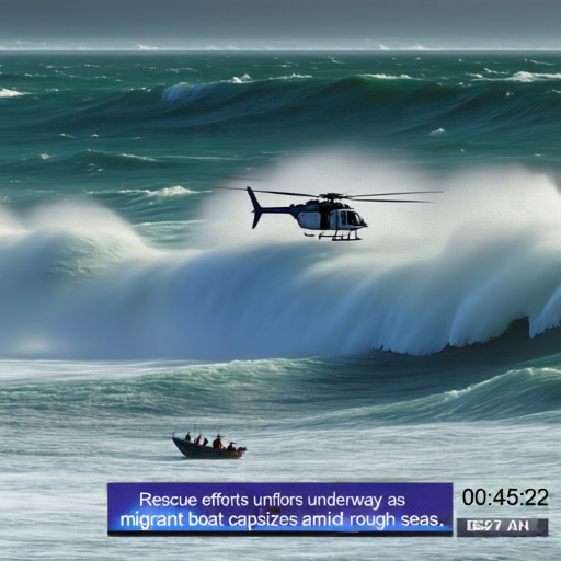


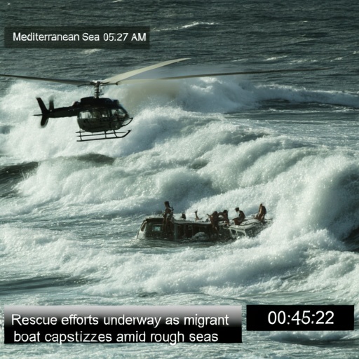

512×512 generations with identical prompts and seeds. AnisoFlow renders finer texture than the \(x\)-prediction baseline (paper, lace, waves, skin) and a sharper, more distinct style than the latent model.
For \(x\)-prediction, recovering the velocity divides the prediction error by \(\sigma_t\), so errors at low noise levels are amplified into visible artifacts, especially under reduced-precision inference. AnisoFlow is trained on the recovered-velocity error directly, so it converges to a well-conditioned target. It stays clean even under 8-bit inference.
Conceptually, the rotate-then-scale form of AnisoFlow’s recovery resembles rotation-based quantization methods. These methods operate layer-wise on an already trained network, whereas AnisoFlow learns the preconditioning end-to-end for the entire network.
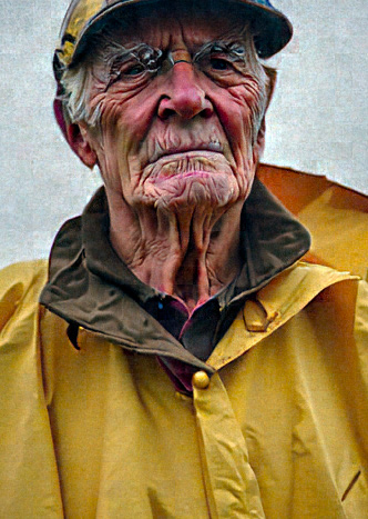
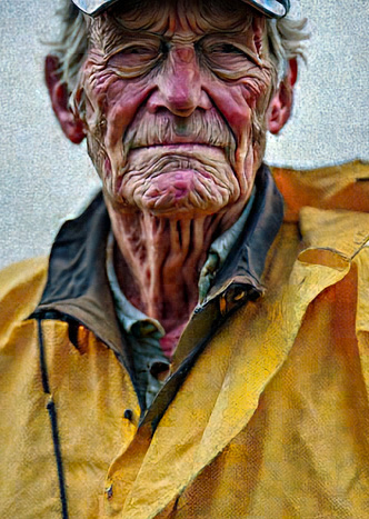
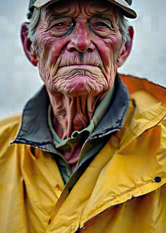


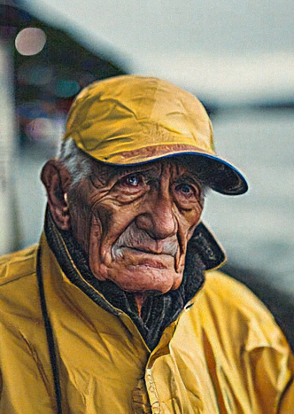
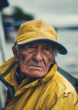


W8A8 inference with the same prompt and seed. \(x\)-prediction develops strong noise or patch seams, while AnisoFlow stays clean.
@article{zirvi2026anisotropic,
  title={Learning Anisotropic Prediction Targets for Flow Models},
  author={Rayhan Zirvi and Hansheng Chen and Gordon Wetzstein and Leonidas Guibas},
  journal={arXiv preprint arXiv:2611.17767},
  url={https://arxiv.org/abs/2611.17767},
  year={2026},
}